Can Passes Become Clues? : Prediction Models Using EPL Passing Networks

Soccer in the Data
Soccer, like many other team sports, thrives on effective passing. A well-executed pass can be the difference between a swift counterattack that leads to a goal and a wasted possession that hands momentum to the opposing team. Although only goals and assists directly determine winners and losers, the additional statistics shed light on each team’s style, organization, and tactical approach. In the English Premier League (EPL), after each match, analysts compile a range of data—goals, assists, possession, fouls, corners, expected goals (xG), expected assists (xA), pass and more. With the continual advancement of Multiple Object Tracking (MOT) technology, even more soccer data will become available, paving the way for deeper investigations into how team tactics can impact performance.
While researching soccer-related data, I stumbled upon Football Passing Networks (https://grafos-da-bola.netlify.app/), a website offering a trove of visualized passing network data. Fascinated by how these networks could illustrate team strategies, I asked myself:
“Can passing networks alone help us forecast which team will win?”
From that spark of curiosity, I centered my analysis on the 2017–2018 English Premier League (EPL) season. I pulled relevant match data(375 matches of EPL 17–18) from the project’s GitHub repository: https://github.com/rodmoioliveira/football-graphs.
Seven Passing Networks: A Tactical Breakdown
To capture the complexity of team play, I subdivided each match’s passing data into seven distinct networks:
- Network 1 (Overall Network)
Considers every “accurate” pass recorded for both teams.
- Network 2 (FW–FW)
Focuses on passes solely among Forwards (FW).
- Network 3 (FW–MD)
Includes passes between Forwards (FW) and Midfielders (MD).
- Network 4 (FW–DF)
Tracks passes between Forwards (FW) and Defenders (DF).
- Network 5 (MD–MD)
Involves passes solely among Midfielders (MD).
- Network 6 (MD–DF)
Comprises passes between Midfielders (MD) and Defenders (DF).
- Network 7 (DF–DF)
Restricts analysis to passes among Defenders (DF).
My reasoning was that each pairing (e.g., FW–MD vs. MD–DF) can highlight unique tactical behaviors. For example, heavy reliance on FW–DF passes might reveal a team that bypasses midfield or regularly launches long balls from defense to attack.
A Closer Look: High-Scoring and Draw Matches
Before diving into network analysis, I examined passing networks from selected matches. I chose games from the 2017–2018 season that featured either significant victory margins or a high total number of goals. Then, I compared the winning and losing teams' passing networks side by side. The row highlighted in yellow in each set of networks indicates the winning team.
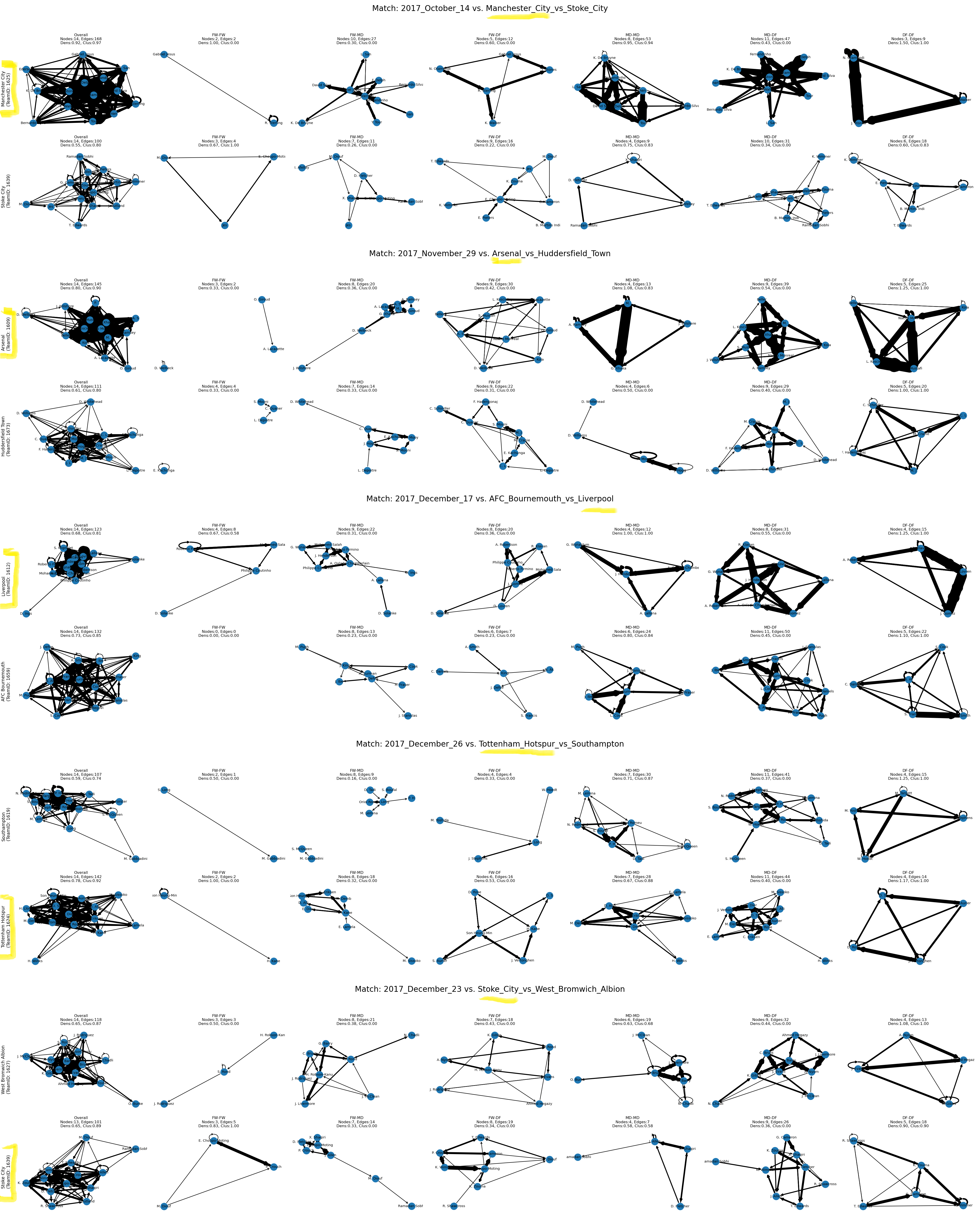
A straightforward way to visually compare passing networks is to look at network density.
- 1. Manchester City vs. Stoke City (7:2)
Clear dominance by Manchester City; in every network (FW–FW, MD–DF, etc.), City showed higher density.
- 2. Arsenal vs. Huddersfield Town (5:0)
Arsenal’s networks were notably denser, aside from FW–FW (which was equal for both teams).
- 3. AFC Bournemouth vs. Liverpool (0:4)
Liverpool dominated nearly all sub-networks, but AFC Bournemouth oddly had a higher overall passing density, demonstrating that a team can connect more passes yet fail to convert them into threatening moves.
- 4. Tottenham Hotspur vs. Southampton (5:2)
Tottenham displayed generally denser passing networks, though Southampton did surpass Spurs in DF–DF and MD–MD.
- 5. Stoke City vs. West Bromwich Albion (3:1)
Stoke’s sub-networks were usually less dense, except for FW–FW, which showed slightly more activity.
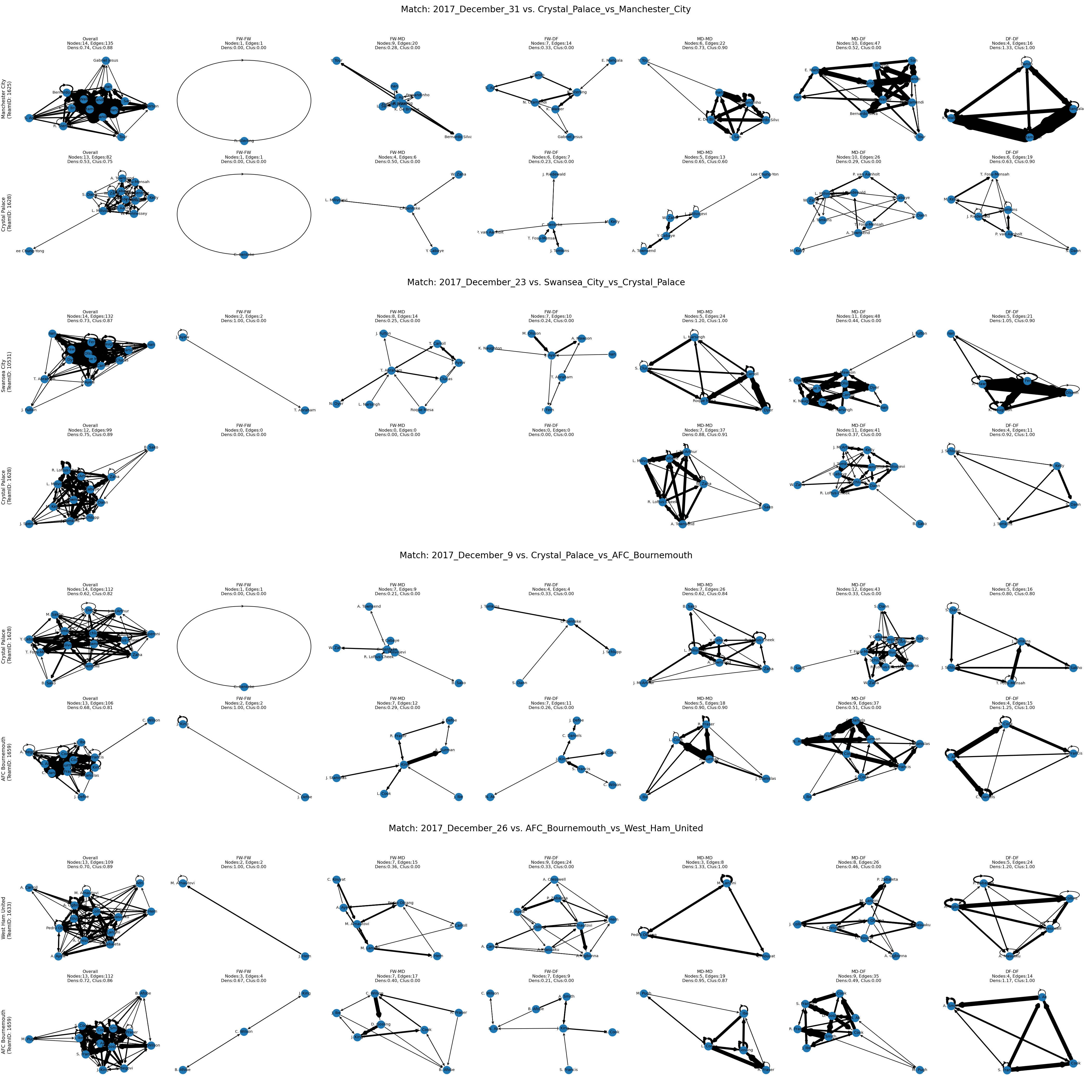
What about matches that ended in a draw?
- 1. Crystal Palace vs. Manchester City (0:0)
- 2. Swansea City vs. Crystal Palace (1:1)
- 3. Crystal Palace vs. AFC Bournemouth (2:2)
- 4. AFC Bournemouth vs. West Ham United (3:3)
In the first match, Manchester City exhibited higher overall network density but failed to translate this advantage into goals. The second match presents a fascinating scenario: despite Crystal Palace not registering any accurate passes between forwards, midfielders, or defenders, Swansea City’s denser network still resulted in a 1:1 draw. In the third and fourth matches, neither team consistently outperformed the other in terms of overall density.
While high passing network density often indicates control and fluidity of play, it doesn't necessarily translate into a decisive victory.
Network Analysis 101: Comparing Structures
To compare networks, we often rely on network metrics like:
- Density (ratio of actual connections to possible connections),
- Transitivity (tendency to form “triangles”),
- Centrality (identifying key players who see the most passes),
- Clustering coefficient, and more.
Tantardini et al. (2019) describes two major categories of network comparison methods. Known Node-Correspondence (KNC) methods use adjacency matrices to directly compare networks, operating under the assumption that the same set of nodes is present in each network. In contrast, Unknown Node-Correspondence (UNC) methods often compare overall network statistics or focus on small sub-networks. These small sub-networks are referred to as graphlets or motifs. Graphlets typically consist of 2–5 nodes, but motifs are structural patterns that appear more frequently than chance would predict.
Li et al. (2015) analyze soccer passing networks by focusing on small sub-networks, specifically 3-node patterns known as motifs. They found that certain motifs occur more frequently in teams with offensive tactics, whereas different motifs are prevalent in teams employing defensive strategies. Their research linked these motif patterns to match outcomes, highlighting which configurations proved more "efficient." In this vein, small sub-networks not only facilitate network comparisons but also offer a valuable lens for analyzing passing strategies. Consequently, this article employs graphlets—small sub-networks—as the basis for its analysis.
Prediction Models Using Graphlet Correlation Distance (GCD-11)
Graphlet Correlation Distance (GCD-11) can be used to compare local connectivity patterns of two undirected networks. Graphlets capture detailed information about a network’s microstructure.
Calculating the GCD typically involves two steps:
- Graphlet Degree : This measures how frequently a node is involved in specific structural positions called orbits (distinct node positions in the sub-network). GCD-11 focuses on 11 particular orbits.
- Construct an N×11 matrix (where N is the number of nodes) that logs each node’s orbit involvement. Then compute the correlation between each column.
The Euclidean distance between the resulting correlation matrices reflects how similar or different the local connectivity patterns of two networks are. A shorter distance means more similarity; a larger distance means less similarity.
# GCD-11
import networkx as nx
from pyfglt.fglt import compute, compute_graphlet_correlation_matrix, gcm_distance


def compute_gcd_11(G1: nx.Graph, G2: nx.Graph, empty_diff=100.0) -> float:

# Some passing sub networks have fewer than 3 node. In this case, use density difference to improve the model

if G1.number_of_nodes() < 3 or G2.number_of_nodes() < 3:
    return abs(nx.density(G1) - nx.density(G2))

try:
    df_counts1 = compute(G1, raw=False)
    df_counts2 = compute(G2, raw=False)
    gcm1 = compute_graphlet_correlation_matrix(df_counts1, method='spearman')
    gcm2 = compute_graphlet_correlation_matrix(df_counts2, method='spearman')
    distance = gcm_distance(gcm1, gcm2)


# If the computed distance is NaN, use default value = 0

    if np.isnan(distance):
        return 0.0
    return distance
except Exception as e:
    print(f"Error computing GCD-11: {e}")
    return 0.0
Using a Python library called pyfglt, I defined a compute_gcd_11 function to calculate this GCD between the sub-networks of two teams.
However, when a sub-network had fewer than three nodes (e.g., if a team had zero or only one FW, making FW–FW or FW–DF essentially nonexistent),
it was impossible to compute GCD accurately. In those instances, I substituted density differences or assigned 0 if no valid edges existed.
Model Analysis: Logistic Regression vs. Random Forest
I ran both Logistic Regression and Random Forest models using GCD as an input feature:
# Logistic Regression and Random Forest

from sklearn.linear_model import LogisticRegression
from sklearn.model_selection import train_test_split, cross_val_score
from sklearn.ensemble import RandomForestClassifier
# Train data : 300, Test data : 75

# Logistic Regression model
l_model = LogisticRegression()
l_model.fit(X_train, y_train)
y_pred_l = l_model.predict(X_test)
acc_l = accuracy_score(y_test, y_pred_l)

# Random Forest model
r_model = RandomForestClassifier(n_estimators=300, random_state=111)
r_model.fit(X_train, y_train)
y_pred_r = r_model.predict(X_test)
acc_r = accuracy_score(y_test, y_pred_r) 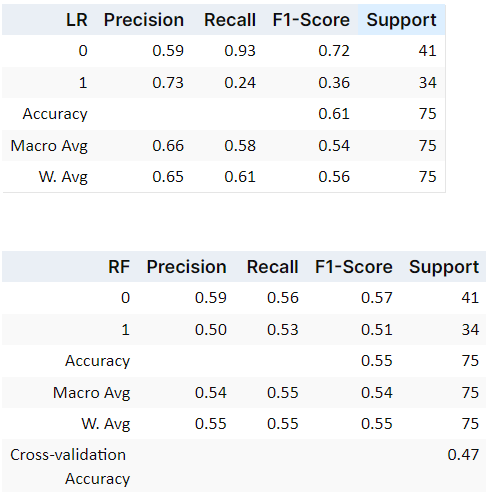
I evaluated two classification models using GCD-based features: Logistic Regression and Random Forest. Logistic Regression achieved approximately 61% overall accuracy. Although the overall accuracy was modest, it excelled in identifying “Non-home team wins” (labeled as 0), with a recall of 0.93. In contrast, the Random Forest model reached only 55% accuracy and a lower cross-validation score of 0.47, suggesting that it overfit the training data and lacked consistency, likely because data is too noisy.
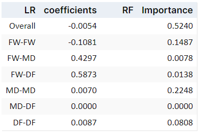
Examining the Logistic Regression coefficients revealed: FW–DF and FW–MD passing networks were the most influential for predicting a non-home team win, implying that strong forward play (connecting with defenders or midfielders) might be crucial in away victories.
Limitations and Future Directions
- Over-Subdivision : Splitting into seven networks occasionally creates sub-networks that are too small to analyze (e.g., only two or three passes total). Future work might experiment with alternative subdivisions or use a single comprehensive passing network.
- Missing Key Variables : Players’ injuries, form, tactical shifts, set-piece strength (corners, free kicks), and refereeing decisions significantly affect matches. Since passing networks alone can’t capture these, incorporating more comprehensive match data could enhance predictive power. In the same context, as discussed in the visualized passing networks comparisons, passing networks can reflect a team’s control and fluidity of play; however, they do not guarantee a decisive victory. This underscores the inherent limitations of using passing networks as sole predictors.
- Time-Dependent Tactics : Passing networks evolve over a 90-minute match as coaches adjust formations, press differently, or chase goals. A temporal or time-series perspective—mapping how passing patterns change minute by minute—could unravel deeper tactical insights.
Still, passing networks are an excellent sandbox for network analysis in sports. They provide ample opportunities to link detailed micro-structures (like graphlets) to strategic decisions on the field.
A Final Word
While passing networks alone may not be the crystal ball of match predictions, they capture vital elements of teamwork and style. Leveraging advanced methods like GCD-11, combined with more traditional metrics (e.g., possession, shots on target), has the potential to deepen our understanding of the tactical layers of soccer. In the grand puzzle of sports analytics, passing networks are one essential piece—and an endlessly fascinating one at that.
References
Li, M.-X., Xu, L.-G., & Zhou, W.-X. (2025). Motif analysis and passing behavior in football passing networks. Chaos, Solitons & Fractals, 190, 115750.
Mói, Rodolfo. Football Passing Networks. Retrieved March 12, 2025, from https://grafos-da-bola.netlify.app/
Tantardini, M., Ieva, F., Tajoli, L., & Piccardi, C. (2019). Comparing methods for comparing networks. Scientific Reports, 9(1), 17557.