The Important thing is whether It’s More Intuitive : Bayesian or Frequentist
The Concept That Lasts Only a Week in Your Mind: Confidence Intervals
If asked, “What’s the biggest advantage of learning Bayesian statistics?” my quick answer would be:
“You can finally let go of the vague and often perplexing concept of confidence intervals.”
One of the earliest challenges for students learning statistical methods is grasping confidence intervals.
Because the concept isn’t intuitive, many forget it soon after their exam(probably within a week).
Typically, the only thing they recall is the number 95%.
Students are taught that “95% of confidence intervals contain the true mean,”
yet what they actually remember is “There’s a 95% chance the true mean lies within the interval.”
While this latter interpretation is technically wrong in the frequentist framework, it’s far more intuitive and aligns with how we naturally think.
Despite efforts to teach the formal definition, what sticks in students’ minds is the more intuitive version.
If this resonates with your own experience, then I say:
“Welcome to Bayesian statistics.”
Why Bayesian Statistics Feels More Intuitive
When we say, “There’s a 95% probability that a parameter lies in the interval,” we’re talking about the credible interval in Bayesian statistics. Although it serves a function similar to the confidence interval, its name and interpretation differ.
What causes this difference?
It largely stems from the frequentist viewpoint.
In frequentist statistics, probabilities arise from the data itself, under the assumption that the dataset collected is one of many potential outcomes.
Analyzing parameters and testing hypotheses with that data is straightforward,
but interpreting those results requires revisiting the probabilistic nature of the dataset.
This back-and-forth hampers intuitive understanding.
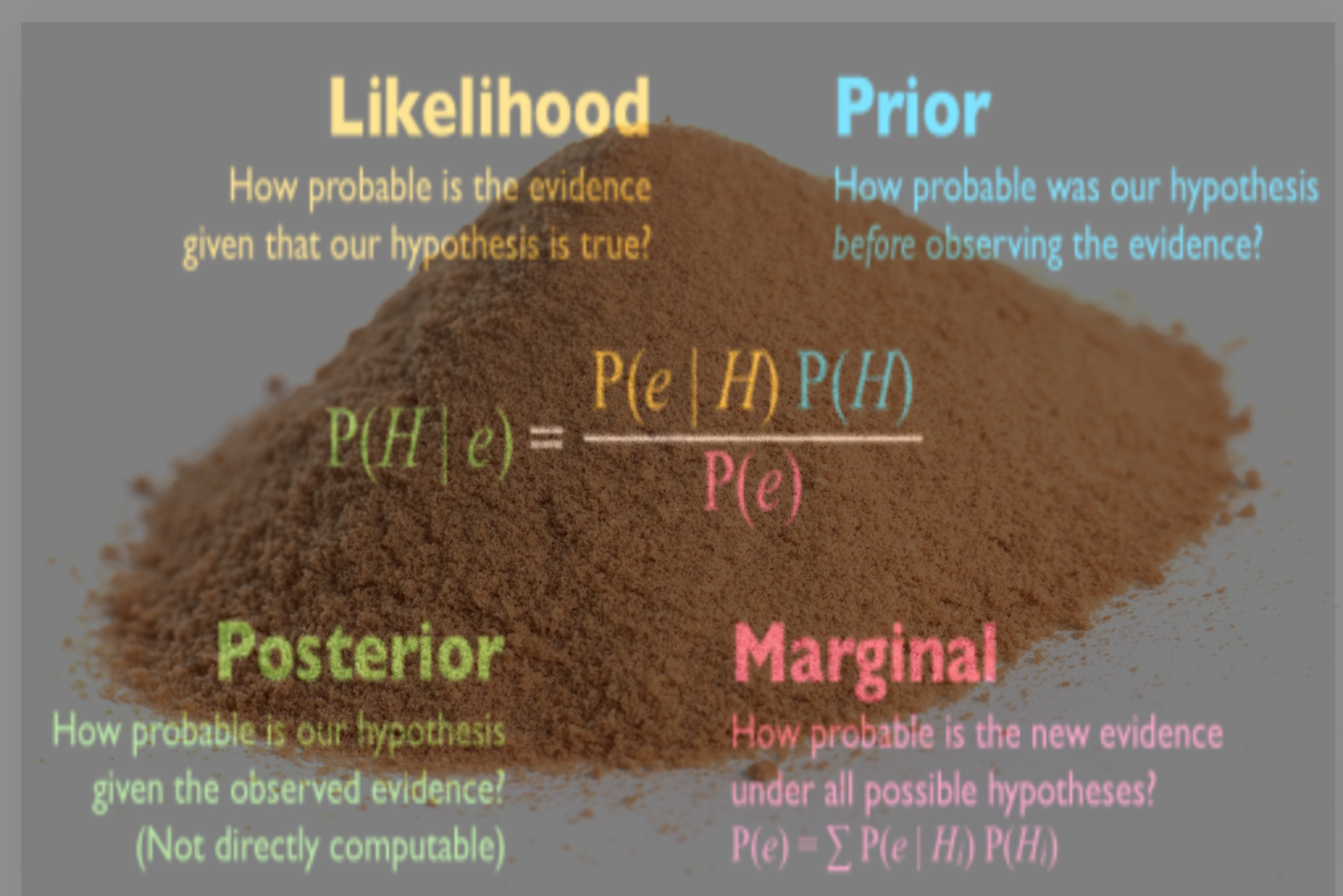
By contrast, Bayesian statistics directly assigns probabilities to parameters. The prior distribution already contains a probability description of the parameter, and the posterior distribution is the revised version of the prior, updated to incorporate the observed data. Unlike frequentist methods, Bayesian interpretation does not demand toggling between data probabilities and parameter probabilities.
The Big Difference that Intuitiveness Can Make : Decision-Making
Imagine assessing a new treatment (T) against a standard treatment (S) for a certain disease, with data from 10 patients in each group:
- New Treatment (T) : 8 out of 10 patients show improvement (Pt = 0.8)
- Standard Treatment (S) : 7 out of 10 patients show improvement (Ps = 0.7)
Frequentist Interpretation
Using the standard error formula:
$$
SE = \sqrt{\frac{0.8 \times 0.2}{10} + \frac{0.7 \times 0.3}{10}} = 0.183
$$
We build a 95% confidence interval (CI) for the difference, Delta = Pt - Ps:
$$
\Delta \pm 1.96 \times 0.183 \;\longrightarrow\; (-0.26,\, 0.46)
$$
Because this interval includes zero, the conclusion is that there’s no statistically significant difference between the treatments.
Bayesian Interpretation
Under the Bayesian framework,
we use a Beta distribution as the prior because the treatment proportion(data) has a binary outcome (success/failure),
which follows a binomial distribution. The Beta distribution is the conjugate prior for the binomial distribution.
This conjugacy means that when the prior is a Beta distribution and the observed data follows a binomial distribution,
the updated posterior will also have the form of a Beta distribution.
Since we have no existing knowledge about the treatments, we pick an uninformative prior,
Beta(1,1) (uniform distribution). When data is applied to the prior :
$$
p_t∣D∼Beta(1+8,1+2)=Beta(9,3)
$$
$$
p_s∣D∼Beta(1+7,1+3)=Beta(8,4)
$$
Then we calculate the posterior distribution of Delta using R:
 # Monte Carlo Simulation for Posterior
N <- 10000

pt <- rbeta(N, 9, 3)
ps <- rbeta(N, 8, 4)

delta <- pt - ps

# 2.5th and 97.5th percentiles
credible_interval <- quantile(delta, probs = c(0.025, 0.975))

print(credible_interval)

>>
      2.5%      97.5%
-0.2733856     0.4263714
In Bayesian statistics, since probabilities are directly assigned to parameters, we can ask:
Even if two treatments are statistically indistinguishable, what is the probability that,
in a simulation comparing a group receiving the new treatment to one receiving the standard treatment, the new treatment performs better?
In other words, what is the probability that Δ>0 ?
mean(delta > 0)
>>
0.6878 Defending the “Less Intuitive” Prior in Bayesian Thinking
In the context of decision-making, it might be more fitting to call the subject Bayesian reasoning rather than Bayesian statistics.
Regardless of the label, the core process remains unchanged: the prior distribution is updated with observed data to create the posterior distribution.
A recurring debate in Bayesian methods centers on selecting the appropriate prior. Which one should we choose?
While this decision is crucial, it also raises the question of why priors often seem so challenging.
Like confidence intervals, priors can feel less intuitive and difficult to grasp.
Why is this so?
At its essence, a prior represents our existing knowledge or belief.
When asked, “Do ghosts exist?” the answer from the repondent's belief is typically a simple yes or no—a binomial outcome.
A question like “Does the advancement of AI contribute to democracy?” can elicit a range of responses—from “yes” to “no,”
with varying degrees of certainty—forming a multinomial framework.
Without imposing a binomial or multinomial structure, converting people’s beliefs into a statistical distribution becomes
a daunting task that only grows more complex with more intricate questions.
Moreover, can we fully trust our knowledge and beliefs?
Humans tend to overestimate dramatic risks while underestimating common ones, and the way information is presented—known as framing effects—can heavily influence our judgments.
Another concern is the reliability of updating priors with new information.
According to Madsen (2016), American voters are more likely to support a policy based on whether particular political figures endorse or criticize it.
In other words, voters’ priors can affect how they interpret new data.
These challenges arise from the inherently less intuitive nature of priors.
Ultimately, priors are subjective probability assessments that naturally vary among individuals, groups, and researchers—and that’s exactly how it should be.
The idea that everyone shares the same knowledge and beliefs is not only unrealistic, it would be quite unsettling.
To illustrate priors further, consider the paradox of the heap.
Imagine a large heap of sand. Removing one grain still leaves you with a heap, but if you continue removing grains until only one remains, is it still a heap?
There is no clear boundary, and different people might answer this question differently.
If we abandon the search for clear boundaries and change our perspective, the paradox of the heap ceases to be a paradox.
Picture a million grains of sand—your confidence that this forms a heap is high.
As you remove one grain at a time, your confidence diminishes gradually.
In this way, belief is not binary but a matter of graded confidence or degrees of belief.
When we think of belief as akin to the confidence that a pile of sand is a heap—decreasing gradually
with each removed grain—priors can indeed become more intuitive.
A belief about any issue can fluctuate like temperature: new data may raise or lower our confidence incrementally.
Different priors(as graded beliefs) can lead to similar or divergent posteriors based on the observed data.
When the evidence is strong, the posterior tends to closely follow the data.
However, if the balance between the prior and the data is maintained, the posterior remains influenced by the priors.
Ultimately, the most appropriate prior is the one that enhances future predictions.
The strength of our subjective priors depends on their ability to predict future outcomes — a process at the very heart of Bayesian reasoning.
Bayesian reasoning helps us find better priors—echoing George Box’s timeless remark:
"All models are wrong, but some are useful."
Reference
Chivers, T. (2024). Everything is Predictable: How Bayesian Statistics Explain Our World. Simon and Schuster.
Fornacon-Wood, I., Mistry, H., Johnson-Hart, C., Faivre-Finn, C., O’Connor, J. P. B., & Price, G. J. (2022). Understanding the Differences Between Bayesian and Frequentist Statistics. International Journal of Radiation Oncology, Biology, Physics, 112(5), 1076–1082.
Madsen, J. K. (2016). Trump supported it?! A Bayesian source credibility model applied to appeals to specific American presidential candidates’ opinions. In Proceedings of the Annual Meeting of the Cognitive Science Society (Vol. 38).